本篇文章由 VeriMake 旧版论坛中备份出的原帖的 Markdown 源码生成
原帖标题为:如何使用 TensorFlow Object Detection API 训练和使用目标检测模型
原帖网址为:https://verimake.com/topics/125 (旧版论坛网址,已失效)
原帖作者为:karb0n(旧版论坛 id = 39,注册于 2020-05-04 19:27:42)
原帖由作者初次发表于 2020-08-01 03:18:16,最后编辑于 2020-08-01 03:18:16(编辑时间可能不准确)
截至 2021-12-18 14:27:30 备份数据库时,原帖已获得 2212 次浏览、0 个点赞、0 条回复
引言
本文以使用 TT100K 数据集训练一个交通标志目标检测器为例,对如何使用 TensorFlow Object Detection API 训练模型和进行目标检测做了一些简单介绍。当然,你也可以自己拍摄或者搜寻其它图片,使用 LabelImg 对图片进行标注,然后仿照本文教程来训练一个能够检测其它物体的目标检测器。
本文分两个部分,第一部分是训练,第二部分是预测。如果你使用的设备的 GPU 显存不大 (例如 < 6 GiB),或者甚至直接使用 CPU 版本的 TensorFlow,可能无法正常进行训练,但是你可以上网搜寻并下载前人们预训练好的模型文件来进行预测,用于预测的代码可以直接参考第 2.2 节。
目录
- 训练
1.1 下载 TT100K 数据集
1.2 将 JSON 格式的标注文件转为 csv 文件
1.3 生成 TFRecord 文件
1.4 生成 pbtxt 格式的类别命名文件
1.5 下载预训练模型准备进行迁移学习
1.6 开始训练
1.7 完成训练
- 检测
2.1 将训练产生的 .ckpt 文件转换为 .pb 文件
2.2 开始检测
1. 训练
1.1 下载 TT100K 数据集
TT100K 数据集是清华-腾讯联合实验室发布的中国交通标志目标检测数据集,打开 TT100K 数据集的网站,点击“Download the Datasets”,下载数据集 Part1(其它部分无需下载,约 17.8 GiB)即可。
下载完成后解压,可以看到这些文件和文件夹
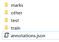
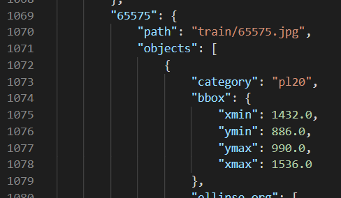
其中,marks 是 TT100K 包含的交通标志类别的示例图片;train 和 test 分别是被拆分出的训练集和测试集;others 是其它一些图片,可以用于训练,也可以用于测试,但是其中的图片不一定每张都包含交通标志;annotations.json 是对数据集的标注文件,里边描述了每张图片里边哪些位置是哪种交通标志,比如下图所示的记录就表示,在图片 train/65575.jpg 中,x∈[1432, 1526], y∈[886, 990] 的矩形范围被标注为 pl20 标签,即这里有个限速20的标志。
1.2 将 JSON 格式的标注文件转为 csv 文件
为便于后续处理,我们编写代码,将 annotations.json 进行处理,将标签转为 train_labels.csv 和 test_labels.csv 两个 csv 文件进行储存。
# -*- coding: UTF-8 -*-
import os
import numpy as np
import json
import csv

splits = ['train', 'test']

for split in splits:
    tt100k_root = 'E:/objDetect/tt100k'  # 这里填你的 TT100K 数据集的根目录

    # 读取 json 文件
    jsonFilePath = os.path.join(tt100k_root, 'data', 'annotations.json')
    with open(jsonFilePath, 'r', encoding='utf-8') as f:
        labels = json.load(f)

    # 读取 ids 文件
    idsFilePath = os.path.join(tt100k_root, 'data', split, 'ids.txt')
    with open(idsFilePath, 'r', encoding='utf-8') as f:
        ids = f.readlines()
        for i in range(len(ids)):
            ids[i] = ids[i].replace('\n','')

    # 将 json 中的标签转换格式,并存于变量 annos 中
    annos = ["filename,width,height,class,xmin,ymin,xmax,ymax"]
    for i in ids:
        for obj in labels['imgs'][i]['objects']:
            anno = "%s.jpg,%d,%d,%s,%f,%f,%f,%f"%(i, 2048, 2048,
                                                  obj['category'],
                                                  obj['bbox']['xmin'],
                                                  obj['bbox']['ymin'],
                                                  obj['bbox']['xmax'],
                                                  obj['bbox']['ymax'])
            annos.append(anno)

    # 把转换格式后的标签写入 csv 文件
    with open('./data/' + split + '_labels.csv','w') as f:
        for anno in annos:
            f.write(anno + '\n')
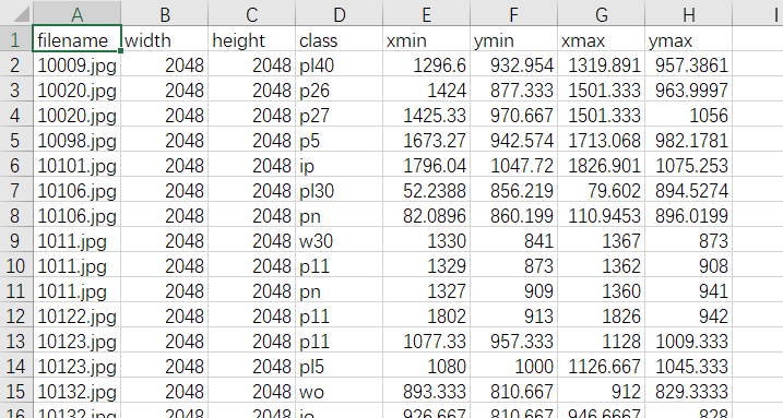
运行完成后,会发现 ./data/ 目录中生成了两个 csv 文件。比如打开 train_labels.csv 文件,我们能看到类似下图的表格,这就是转换格式后的数据集标签。
1.3 生成 TFRecord 文件
TFRecord 是 TensorFlow 提供的一种统一的数据存储格式,相比训练时直接一张一张读取图片文件,使用 TFRecord 进行读取会更加高效。TF OD API 被设计为需要使用 TFRecord 格式读入数据才能够进行训练,所以我们将数据集转换成 TFRecord 格式的文件。
- ConvertCSV2TFRecord.py 的代码
# -*- coding: utf-8 -*-

import os
import io
import pandas as pd
import tensorflow as tf
from PIL import Image
from tqdm import *

os.chdir('E:/objDetect/TensorFlow_OD/models-master/research/')  # 填 TF OD API 上一级的 research 目录的地址
from collections import namedtuple, OrderedDict
from object_detection.utils import dataset_util

# 所有类别的名字
names = ["i1", "i10", "i11", "i12", "i13", "i14", "i15", "i2", "i3", "i4", "i5",
         "il100", "il110", "il50", "il60", "il70", "il80", "il90", "io", "ip", "p1", "p10",
         "p11", "p12", "p13", "p14", "p15", "p16", "p17", "p18", "p19", "p2", "p20", "p21",
         "p22", "p23", "p24", "p25", "p26", "p27", "p28", "p3", "p4", "p5", "p6", "p7", "p8",
         "p9", "pa10", "pa12", "pa13", "pa14", "pa8", "pb", "pc", "pg", "ph1.5", "ph2",
         "ph2.1", "ph2.2", "ph2.4", "ph2.5", "ph2.8", "ph2.9", "ph3", "ph3.2", "ph3.5",
         "ph3.8", "ph4", "ph4.2", "ph4.3", "ph4.5", "ph4.8", "ph5", "ph5.3", "ph5.5",
         "pl10", "pl100", "pl110", "pl120", "pl15", "pl20", "pl25", "pl30", "pl35", "pl40",
         "pl5", "pl50", "pl60", "pl65", "pl70", "pl80", "pl90", "pm10", "pm13", "pm15",
         "pm1.5", "pm2", "pm20", "pm25", "pm30", "pm35", "pm40", "pm46", "pm5", "pm50",
         "pm55", "pm8", "pn", "pne", "po", "pr10", "pr100", "pr20", "pr30", "pr40",
         "pr45", "pr50", "pr60", "pr70", "pr80", "ps", "pw2", "pw2.5", "pw3", "pw3.2",
         "pw3.5", "pw4", "pw4.2", "pw4.5", "w1", "w10", "w12", "w13", "w16", "w18",
         "w20", "w21", "w22", "w24", "w28", "w3", "w30", "w31", "w32", "w34", "w35",
         "w37", "w38", "w41", "w42", "w43", "w44", "w45", "w46", "w47", "w48", "w49",
         "w5", "w50", "w55", "w56", "w57", "w58", "w59", "w60", "w62", "w63", "w66",
         "w8", "wo", "i6", "i7", "i8", "i9", "ilx", "p29", "w29", "w33", "w36", "w39",
         "w4", "w40", "w51", "w52", "w53", "w54", "w6", "w61", "w64", "w65", "w67",
         "w7", "w9", "pax", "pd", "pe", "phx", "plx", "pmx", "pnl", "prx", "pwx",
         "w11", "w14", "w15", "w17", "w19", "w2", "w23", "w25", "w26", "w27", "pl0",
         "pl4", "pl3", "pm2.5", "ph4.4", "pn40", "ph3.3", "ph2.6"]


def class_text_to_int(row_label):
    return names.index(row_label) + 1


def split(df, group):
    data = namedtuple('data', ['filename', 'object'])
    gb = df.groupby(group)
    return [data(filename, gb.get_group(x)) for filename, x in zip(gb.groups.keys(), gb.groups)]


def create_tf_example(group, path):
    with tf.gfile.GFile(os.path.join(path, '{}'.format(group.filename)), 'rb') as fid:
        encoded_jpg = fid.read()
    encoded_jpg_io = io.BytesIO(encoded_jpg)
    image = Image.open(encoded_jpg_io)
    width, height = image.size

    filename = group.filename.encode('utf8')
    image_format = b'jpg'
    xmins = []
    xmaxs = []
    ymins = []
    ymaxs = []
    classes_text = []
    classes = []

    for index, row in group.object.iterrows():
        xmins.append(row['xmin'] / width)
        xmaxs.append(row['xmax'] / width)
        ymins.append(row['ymin'] / height)
        ymaxs.append(row['ymax'] / height)
        classes_text.append(row['class'].encode('utf8'))
        classes.append(class_text_to_int(row['class']))

    tf_example = tf.train.Example(features=tf.train.Features(feature={
        'image/height': dataset_util.int64_feature(height),
        'image/width': dataset_util.int64_feature(width),
        'image/filename': dataset_util.bytes_feature(filename),
        'image/source_id': dataset_util.bytes_feature(filename),
        'image/encoded': dataset_util.bytes_feature(encoded_jpg),
        'image/format': dataset_util.bytes_feature(image_format),
        'image/object/bbox/xmin': dataset_util.float_list_feature(xmins),
        'image/object/bbox/xmax': dataset_util.float_list_feature(xmaxs),
        'image/object/bbox/ymin': dataset_util.float_list_feature(ymins),
        'image/object/bbox/ymax': dataset_util.float_list_feature(ymaxs),
        'image/object/class/text': dataset_util.bytes_list_feature(classes_text),
        'image/object/class/label': dataset_util.int64_list_feature(classes),
    }))
    return tf_example


def convertTFR(img_path, csv_input, output_path):
    writer = tf.python_io.TFRecordWriter(output_path)
    examples = pd.read_csv(csv_input)
    grouped = split(examples, 'filename')
    for group in tqdm(grouped):
        tf_example = create_tf_example(group, img_path)
        writer.write(tf_example.SerializeToString())

    writer.close()
    print('Successfully created the TFRecords: {}'.format(output_path))


if __name__ == '__main__':

    # 转换训练集为TFRecord格式,这里要根据你的图片和csv文件的实际路径来更改
    img_path = 'E:/objDetect/tt100k/data/train/'
    csv_input = 'E:/objDetect/tt100k/data/train_labels.csv'
    output_path = 'E:/objDetect/tt100k/data/TFRecords/train.tfrecord'
    convertTFR(img_path, csv_input, output_path)

    # 转换测试集为TFRecord格式,这里要根据你的图片和csv文件的实际路径来更改
    img_path = 'E:/objDetect/tt100k/data/test/'
    csv_input = 'E:/objDetect/tt100k/data/test_labels.csv'
    output_path = 'E:/objDetect/tt100k/data/TFRecords/test.tfrecord'
    convertTFR(img_path, csv_input, output_path)
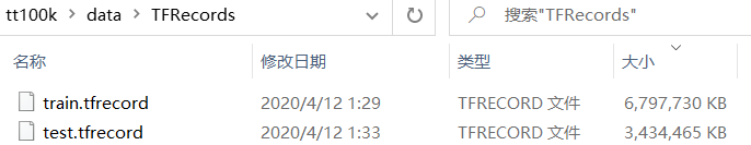
运行此代码,等待一段时间后,即转换完成,可找到下图的两个文件。
1.4 生成 pbtxt 格式的类别命名文件
TF OD API 可通过 pbtxt 格式的文件来读取各个类别对应的名称,我们可以直接使用下边的代码来生成适用于 TT100K 数据集的 pbtxt 文件。
names = ["i1", "i10", "i11", "i12", "i13",
         "i14", "i15", "i2", "i3", "i4",
         "i5", "il100", "il110", "il50", "il60",
         "il70", "il80", "il90", "io", "ip",
         "p1", "p10", "p11", "p12", "p13",
         "p14", "p15", "p16", "p17", "p18",
         "p19", "p2", "p20", "p21", "p22",
         "p23", "p24", "p25", "p26", "p27",
         "p28", "p3", "p4", "p5", "p6",
         "p7", "p8", "p9", "pa10", "pa12",
         "pa13", "pa14", "pa8", "pb", "pc",
         "pg", "ph1.5", "ph2", "ph2.1", "ph2.2",
         "ph2.4", "ph2.5", "ph2.8", "ph2.9", "ph3",
         "ph3.2", "ph3.5", "ph3.8", "ph4", "ph4.2",
         "ph4.3", "ph4.5", "ph4.8", "ph5", "ph5.3",
         "ph5.5", "pl10", "pl100", "pl110", "pl120",
         "pl15", "pl20", "pl25", "pl30", "pl35",
         "pl40", "pl5", "pl50", "pl60", "pl65",
         "pl70", "pl80", "pl90", "pm10", "pm13",
         "pm15", "pm1.5", "pm2", "pm20", "pm25",
         "pm30", "pm35", "pm40", "pm46", "pm5",
         "pm50", "pm55", "pm8", "pn", "pne",
         "po", "pr10", "pr100", "pr20", "pr30",
         "pr40", "pr45", "pr50", "pr60", "pr70",
         "pr80", "ps", "pw2", "pw2.5", "pw3",
         "pw3.2", "pw3.5", "pw4", "pw4.2", "pw4.5",
         "w1", "w10", "w12", "w13", "w16",
         "w18", "w20", "w21", "w22", "w24",
         "w28", "w3", "w30", "w31", "w32",
         "w34", "w35", "w37", "w38", "w41",
         "w42", "w43", "w44", "w45", "w46",
         "w47", "w48", "w49", "w5", "w50",
         "w55", "w56", "w57", "w58", "w59",
         "w60", "w62", "w63", "w66", "w8",
         "wo", "i6", "i7", "i8", "i9",
         "ilx", "p29", "w29", "w33", "w36",
         "w39", "w4", "w40", "w51", "w52",
         "w53", "w54", "w6", "w61", "w64",
         "w65", "w67", "w7", "w9", "pax",
         "pd", "pe", "phx", "plx", "pmx",
         "pnl", "prx", "pwx", "w11", "w14",
         "w15", "w17", "w19", "w2", "w23",
         "w25", "w26", "w27", "pl0", "pl4",
         "pl3", "pm2.5", "ph4.4", "pn40", "ph3.3",
         "ph2.6"]


with open('./tt100k_label_map.pbtxt', 'w') as f:
    for i in range(len(names)):
        temp = "item{\n    id:%d\n    name:\'%s\'\n}\n\n" % (i+1, names[i])
        f.write(temp)

''' LABEL MAP EXAMPLE:

item{
    id:1
    name:'i1'
}

item{
    id:2
    name:'i10'
}

………………

'''
1.5 下载预训练模型准备进行迁移学习
适用于 TF OD API 格式的数据集已经准备完成了,我们可以准备开始训练了。但是呢,从随机初始化开始训练一个现代的目标检测网络,耗时是非常长的。好在,我们能够下载一些使用其它数据集预训练过的模型来进行迁移学习,这样会大大缩短训练所需的时间。
打开 TensorFlow 1 Detection Model Zoo,根据表格中展示的速度和准确度,选择一个你想使用的模型下载。
本文以 faster_rcnn_resnet101_coco 为例,就是使用 MS COCO 数据集 预训练过的 Faster R-CNN with ResNet101 模型。将下载的 faster_rcnn_resnet101_coco_2018_01_28.tar.gz 压缩包解压后,可以得到下图所示的这些文件
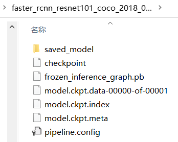
我们把 pipeline.config 复制一份,并重命名(例如 faster_rcnn_resnet101_TSR.config),然后打开重命名后的文件,参照文件中的提示,根据我们数据集的类别数量、TFRecord 和 pbtxt 文件的路径,修改这个文件中的部分内容。
例如,一份示例的 faster_rcnn_resnet101_TSR.config 内容如下:
- faster_rcnn_resnet101_TSR.config 文件内容,其中需要更改的地方被 XXX 标记出
# Faster R-CNN with Resnet-101 (v1), configuration for TT100K Dataset.
# Users should configure the fine_tune_checkpoint field in the train config as
# well as the label_map_path and input_path fields in the train_input_reader and
# eval_input_reader. Search for "PATH_TO_BE_CONFIGURED" to find the fields that
# should be configured.

model {
  faster_rcnn {
    num_classes: 221   # XXX: configure to fit your dataset
    image_resizer {
      keep_aspect_ratio_resizer {
        min_dimension: 600
        max_dimension: 1024
      }
    }
    feature_extractor {
      type: 'faster_rcnn_resnet101'
      first_stage_features_stride: 16
    }
    first_stage_anchor_generator {
      grid_anchor_generator {
        scales: [0.25, 0.5, 1.0, 2.0]
        aspect_ratios: [0.5, 1.0, 2.0]
        height_stride: 16
        width_stride: 16
      }
    }
    first_stage_box_predictor_conv_hyperparams {
      op: CONV
      regularizer {
        l2_regularizer {
          weight: 0.0
        }
      }
      initializer {
        truncated_normal_initializer {
          stddev: 0.01
        }
      }
    }
    first_stage_nms_score_threshold: 0.0
    first_stage_nms_iou_threshold: 0.7
    first_stage_max_proposals: 300
    first_stage_localization_loss_weight: 2.0
    first_stage_objectness_loss_weight: 1.0
    initial_crop_size: 14
    maxpool_kernel_size: 2
    maxpool_stride: 2
    second_stage_box_predictor {
      mask_rcnn_box_predictor {
        use_dropout: false
        dropout_keep_probability: 1.0
        fc_hyperparams {
          op: FC
          regularizer {
            l2_regularizer {
              weight: 0.0
            }
          }
          initializer {
            variance_scaling_initializer {
              factor: 1.0
              uniform: true
              mode: FAN_AVG
            }
          }
        }
      }
    }
    second_stage_post_processing {
      batch_non_max_suppression {
        score_threshold: 0.0
        iou_threshold: 0.6
        max_detections_per_class: 100
        max_total_detections: 300
      }
      score_converter: SOFTMAX
    }
    second_stage_localization_loss_weight: 2.0
    second_stage_classification_loss_weight: 1.0
  }
}

train_config: {
  batch_size: 2  # XXX: configure to fit your GPU, if you have a more powerful GPU, you can try a bigger size
  optimizer {
    momentum_optimizer: {
      learning_rate: {
        manual_step_learning_rate {
          initial_learning_rate: 0.0003
          schedule {
            step: 30000
            learning_rate: .00003
          }
          schedule {
            step: 40000
            learning_rate: .000003
          }
        }
      }
      momentum_optimizer_value: 0.9
    }
    use_moving_average: false
  }
  gradient_clipping_by_norm: 10.0
  fine_tune_checkpoint: "E:/objDetect/tt100k/pretrained-models/faster_rcnn_resnet101_coco_2018_01_28/model.ckpt"  # XXX: configure to fit your dataset
  from_detection_checkpoint: true
  num_steps: 50000
}

train_input_reader: {
  tf_record_input_reader {
    input_path: "E:/objDetect/tt100k/data/TFRecords/train.tfrecord"  # XXX: configure to fit your dataset
  }
  label_map_path: "E:/objDetect/tt100k/data/TFRecords/tt100k_label_map.pbtxt"  # XXX: configure to fit your dataset
}

eval_config: {
  num_examples: 3071  # XXX: configure to fit your dataset
  batch_size: 1  # XXX: configure to fit your GPU, if you have a more powerful GPU, you can try a bigger size
  num_visualizations: 50
  min_score_threshold: 0.3

  # Note: The below line limits the evaluation process to 10 evaluations.
  # Remove the below line to evaluate indefinitely.
  max_evals: 10
}

eval_input_reader: {
  tf_record_input_reader {
    input_path: "E:/objDetect/tt100k/data/TFRecords/test.tfrecord"  # XXX: configure to fit your dataset
  }
  label_map_path: "E:/objDetect/tt100k/data/TFRecords/tt100k_label_map.pbtxt"  # XXX: configure to fit your dataset
  shuffle: false
  num_readers: 1
}
1.6 开始训练
终于把需要用到的文件都准备好了:monkey: ,我们在命令行里进入 research\object_detection\legacy 目录,输入
python train.py --logtostderr --train_dir=E:/objDetect/tt100k/training/ --pipeline_config_path=E:/objDetect/tt100k/faster_rcnn_resnet101_TSR.config
就可以开始训练了。(注意:这行指令中的路径都是需要根据你的实际情况来修改的)
在 GTX 1060 GPU 下需要训练接近 11 个小时,所以在运行前请做好这台电脑十几个小时不能另外使用的准备。
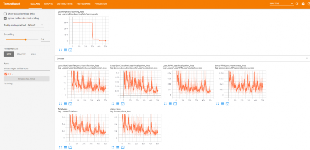
train_dir 指定的路径不仅会储存一些训练过程中的 checkpoint,还包含了能够使用 TensorBoard 观察训练过程的文件,所以,我们另开一个命令行,输入
tensorboard --logdir E:/objDetect/tt100k/training/
即可打开 TensorBoard 来观察我们的训练过程。下图是损失函数的变化图表的一个示例。
1.7 完成训练
出去玩了一圈或者睡一觉醒来之后,可能还没训练好 终于训练好了,我们在 research\object_detection\legacy 目录下,输入
python eval.py --logtostderr --eval_dir=E:/objDetect/tt100k/evaluating/ --pipeline_config_path=E:/objDetect/tt100k/faster_rcnn_resnet101_TSR.config --checkpoint_dir=E:/objDetect/tt100k/training/
就可以使用 TF OD API 自带的功能来进行性能评估,并生成对随机几张示例图片的预测结果。(注意:这行指令中的路径同样是需要根据你的实际情况来修改的)
也是使用 TensorBoard 来查阅评估结果,另开一个命令行,输入
tensorboard --logdir E:/objDetect/tt100k/evaluating/
即可打开 TensorBoard 来查阅训练好的模型的评估结果。下图是一个示例
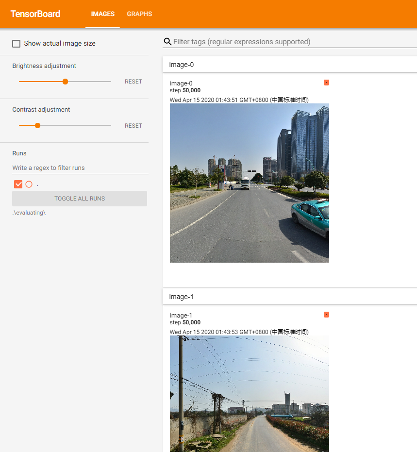
因为 TT100K 数据集里数据分布不太均匀,所以直接进行训练产生的模型准确度可能比较一般。如果评估发现模型对交通标志是有一定的检测能力的,就说明训练是有效的。
2. 检测
2.1 将训练产生的 .ckpt 文件转换为 .pb 文件
.ckpt 文件是训练过程中记录的 checkpoint 文件,我们需要将其转换为 .pb 文件才能在后续进行实际的预测或者部署。
在命令行里进入 research\object_detection 目录,输入
python export_inference_graph.py --input_type image_tensor --pipeline_config_path E:/objDetect/tt100k/faster_rcnn_resnet101_TSR.config --trained_checkpoint_prefix E:/objDetect/tt100k/training/model.ckpt-50000 --output_directory E:/objDetect/tt100k/TSRmodels
等待运行完成后,即转换完成。(注意:这行指令中的路径都是需要根据你的实际情况来修改的)
2.2 开始检测
参考下列代码,修改其中的一些文件地址,运行,即可对一张图片进行交通标志目标检测。也可以使用 cv2.VideoCapture 来进行对视频流(视频文件或者摄像头均可)的检测。
#!/usr/bin/env python
# -*- coding: utf-8 -*-
import os
import sys
import cv2
import numpy as np
import tensorflow as tf
from object_detection.utils import label_map_util
from object_detection.utils import visualization_utils as vis_util
from PIL import Image
import matplotlib
import matplotlib.pyplot as plt
matplotlib.use('Qt5Agg')
# Path to frozen detection graph. This is the actual model that is used for the object detection.
PATH_TO_CKPT = 'E:/objDetect/tt100k/TSRmodels/20200414_faster_rcnn_resnet101_TSR.pb'
# List of the strings that is used to add correct label for each box.
PATH_TO_LABELS = 'E:/objDetect/tt100k/data/TFRecords/tt100k_label_map.pbtxt'
# 分类数量
NUM_CLASSES = 221
detection_graph = tf.Graph()
with detection_graph.as_default():
od_graph_def = tf.GraphDef()
with tf.gfile.GFile(PATH_TO_CKPT, 'rb') as fid:
serialized_graph = fid.read()
od_graph_def.ParseFromString(serialized_graph)
tf.import_graph_def(od_graph_def, name='')
label_map = label_map_util.load_labelmap(PATH_TO_LABELS)
categories = label_map_util.convert_label_map_to_categories(
label_map, max_num_classes=NUM_CLASSES, use_display_name=True)
category_index = label_map_util.create_category_index(categories)
with detection_graph.as_default():
with tf.Session(graph=detection_graph) as sess:
image = cv2.imread("./7433.jpg")
# Expand dimensions since the model expects images to have shape: [1, None, None, 3]
image_np_expanded = np.expand_dims(image, axis=0)
image_tensor = detection_graph.get_tensor_by_name(
'image_tensor:0')
# Each box represents a part of the image where a particular object was detected.
boxes = detection_graph.get_tensor_by_name(
'detection_boxes:0')
# Each score represent how level of confidence for each of the objects.
# Score is shown on the result image, together with the class label.
scores = detection_graph.get_tensor_by_name(
'detection_scores:0')
classes = detection_graph.get_tensor_by_name(
'detection_classes:0')
num_detections = detection_graph.get_tensor_by_name(
'num_detections:0')
# Actual detection.
(boxes, scores, classes, num_detections) = sess.run(
[boxes, scores, classes, num_detections],
feed_dict={image_tensor: image_np_expanded})
# Visualization of the results of a detection.
vis_util.visualize_boxes_and_labels_on_image_array(
image,
np.squeeze(boxes),
np.squeeze(classes).astype(np.int32),
np.squeeze(scores),
category_index,
min_score_thresh=0.4,
use_normalized_coordinates=True,
line_thickness=8)
result = np.asarray(image)
plt.imshow(cv2.cvtColor(result, cv2.COLOR_BGR2RGB))
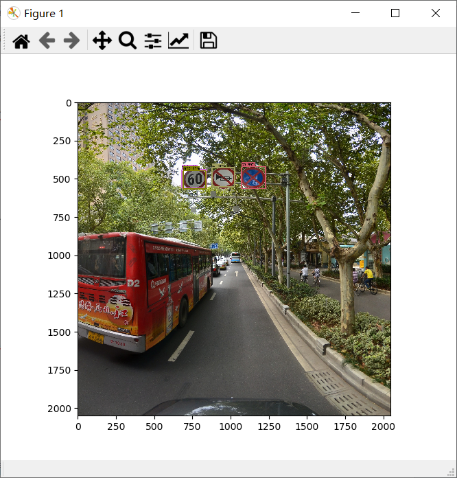
plt.show()
运行上边代码会显示下边这张图,可以看出,它能够成功检测出这张图片出的三个交通标志。
 网站备案号:ICP备16046599号-1